How wide should your liquidity range be?

We published this piece and then broke it ourselves, the same day. The original version concluded that narrow ranges won decisively on our WETH/USDC pool and lost on our cbBTC/USDC one, and that the two pools therefore gave opposite answers. That conclusion rested on a number we had assumed rather than measured: how tightly the existing liquidity sits around the current price.

We then measured it, on that exact pool, against the real fees a real position captured on-chain. It came out roughly nine times smaller than we had assumed. With the measured value, the WETH result inverts: narrow ranges go from clearly winning to clearly losing, and buy and hold wins instead.

So narrow did not beat wide in either pool, and the "opposite answers" framing was wrong. The rest of the piece stands, and the lesson got sharper rather than weaker: we wrote an article about measurement beating assumption, and the conclusion was being carried by our own unmeasured assumption. The sections below are the corrected version; this note stays permanently.

Concentrated liquidity gives you one big lever: how wide a price band you deposit into. Everybody knows the first-order effect. A narrower band earns more fees per dollar deposited, because your capital is stacked where the trading actually happens. A wider band earns less per dollar, but the price wanders out of it far less often.

The part that gets skipped is that both sides of that trade scale, and they do not scale together. Narrowing the band multiplies your fee income by roughly the factor you narrowed it. It also multiplies how often the price leaves your range, how often you rebalance, and how much inventory you are forced to swap at the worst possible moment. The first is a gain that scales with what the pool pays you. The second is a cost that scales with how much the asset moves.

Which means the answer cannot be a number. It is a comparison between two quantities that have nothing to do with each other: the pool's fee yield, and the asset's volatility. Change either and the answer flips.

We size ranges from measured volatility rather than from a fixed percentage, so "narrow" and "wide" are multipliers on a volatility estimate, not constants. Across the eight years of price history in this test, that works out to these typical half-widths:

• Narrow is a band of about ±16% on the BTC-quoted pool and ±22% on the ETH-quoted one. This is the range family real LPs actually use.
• Wide is eight times that: roughly ±127% and ±173%. At that width the price essentially never leaves, and the position behaves close to simply holding the two assets.

We also carry a plain buy and hold of the same two assets through every test, because a strategy that cannot beat holding the tokens has not earned the complexity it costs.

Everything below is out-of-sample. We cut the price history into consecutive folds: one year of training, then the following 90 days as a test window that the strategy never saw. Slide forward, repeat. Each window runs as an independent backtest with its own 90-day lead-in, so the volatility estimate that sizes the range is always causal and never peeks at the future.

That gives 29 test folds, running from April 2019 to May 2026: eight years spanning two bull markets, two brutal drawdowns and a lot of sideways. The pool's own swap fee is charged on every rebalance that trades inventory, so narrow ranges pay for their own churn rather than rebalancing for free.

We report Sharpe ratio rather than total return, and there is a reason for that which matters later: these runs hold the fee level constant for eight years, which no real pool does. That assumption is harmless for comparing strategies against each other in the same run, and useless for predicting how much money anything makes.

The first pool is a cbBTC/USDC pool on Base. We measure what it actually pays by reading the fee accumulator on-chain rather than trusting a listed APR, and across 38 measurements its median swap fee yield on unstaked liquidity is about 13 percent a year.

At that fee level, over 29 out-of-sample folds:

• Narrow, keeping whatever inventory the market leaves you: Sharpe −0.49
• Narrow, rebalancing back to a 50/50 split: Sharpe −0.03
• Wide: Sharpe 0.64
• Buy and hold: Sharpe 0.77

Narrow ranges are not merely worse than wide ones here. They are worse than not providing liquidity at all. Thirteen percent a year, multiplied up by concentration, still does not cover what the churn costs on an asset this volatile. The fees are real and they are simply not enough.

This one stung, because it contradicted our own earlier conclusion. In 2024 we had this same pool as evidence that narrow ranges win, and it was, at the fee level we believed at the time, which was 34 percent. That figure came from an aggregator. When we started measuring the chain ourselves it turned out to be closer to 13, and the finding died with the number that produced it.

The second pool is a WETH/USDC pool on the same chain, same protocol, tested the same week. Its measured median across 37 readings is about 51 percenta year, roughly four times the first pool's, on an asset that is more volatile, not less.

This is the pool the correction is about. Our first version ran it with an assumed concentration: how tightly the existing liquidity sits around the current price. We had no measurement for this pool, so we used the value generally quoted for the pair, 0.50. On that assumption, narrow won decisively: Sharpe 1.44 against 0.94 for wide and 0.81 for holding.

Then we measured it properly, by inverting the model against the fees a real position in that pool actually captured on-chain over eight days. The measured value is about 0.056, roughly nine times smaller. Same test, same 29 folds, with the measured concentration instead of the assumed one:

• Narrow, rebalancing to 50/50: Sharpe −0.48 (was +1.44)
• Narrow, keeping inventory: Sharpe −0.87 (was +1.16)
• Wide: Sharpe 0.58 (was 0.94)
• Buy and hold: Sharpe 0.81 (unchanged, it does not depend on this)

A tighter real concentration means the existing liquidity is stacked more densely where you want to sit, so your share of the fee flow is smaller than the model assumed. The direction of the whole result turns on it. Narrow does not win here either.

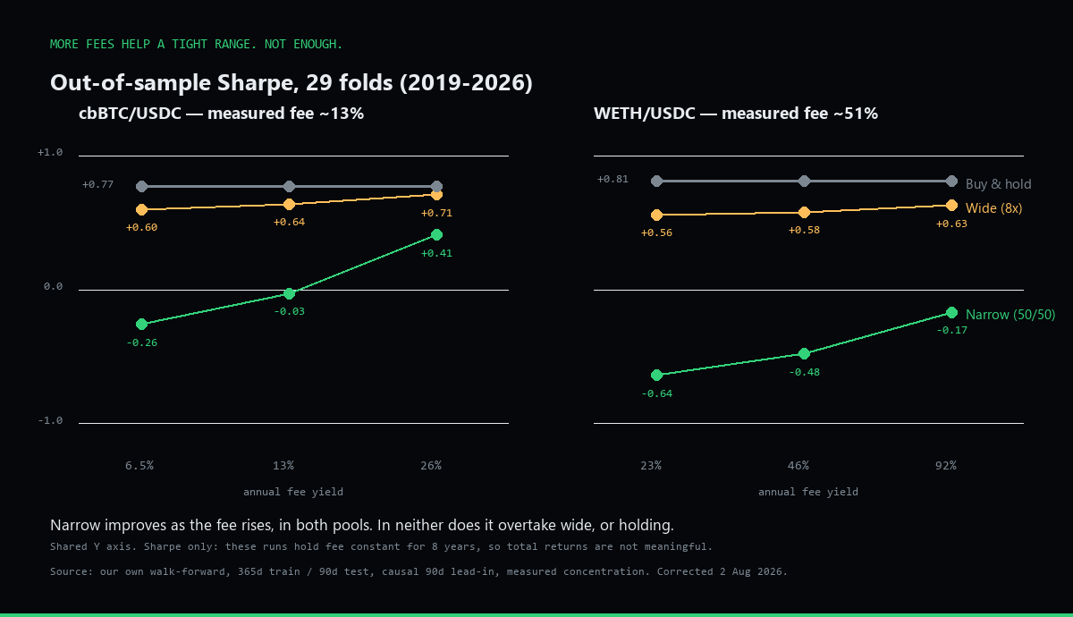
To find out what drives the answer, we swept each pool at half its measured fee, at its measured fee, and at double, holding everything else fixed. The fee level does move the result, in the direction you would expect. It just does not move it far enough.

In the BTC-quoted pool, narrow climbs steadily as the fee rises: from −0.26 at half fee, to −0.03 at measured fee, to 0.41 at double, but never catches the wide range, which sits between 0.60 and 0.71 the whole way. In the ETH-quoted pool the shape is the same: −0.64, −0.48, −0.17, always below the wide range and always below holding.

So the fee level genuinely is a lever, and it points the way everyone expects: more fees, better case for a tight range. But in both of our pools, at the fees they actually pay and at double those fees, the crossover is never reached. On this evidence a tight range needs considerably more than these pools pay before it earns the churn it causes.

The width question, then, is downstream of two measurement questions, not one. What does this pool actually pay, and how tightly is its liquidity already packed. We had measured the first and assumed the second, and it was the second that decided the answer.

We would rather state the limits than have them found for us.

Ignore the returns; only the ordering is meaningful. These runs hold the fee level fixed for eight years and compound it. At the higher fee levels that produces total returns in the thousands of percent, which are an artefact of the assumption and not a forecast of anything. We are publishing the relative ranking of strategies within each run, and deliberately not publishing the magnitudes.

Buy and hold is flattered by the period. 2018 to 2026 was net strongly bullish for both assets. A liquidity position is structurally short volatility, so it lags a rising market by construction. In a flat or falling stretch the comparison looks very different, and that is a property of the window, not a defect of the pools.

The concentration measurement is thin, and it is the number that decided everything. The cbBTC figure has been calibrated on-chain for a while. The WETH one is new, and it comes from a single real position over eight days: eight daily intervals, with individual readings ranging from 0.016 to 0.089 around a median of 0.056. That is a wide spread and we are not presenting it as settled. What we can say is that the conclusion does not hinge on where inside that range the true value sits: even at the most favourable end, narrow stays far below where the assumed 0.50 had put it. We are gathering more data and a second, independent method of measuring it.

Costs are modelled, but not all of them.The pool's swap fee is charged on every rebalance. Slippage is not modelled at all, which means narrow ranges, the strategies that rebalance most, get a small free pass they would not get in production.

And the fee is a measurement of the past, not a promise. Everything above says what these pools have paid. Neither of those numbers is a commitment to keep paying it, and a pool crossing back over the line would invert its own answer.

The practical consequence is that we do not carry a house range width. The width has to be a function of what the pool pays, how much the asset moves, and how crowded the pool already is, recomputed as those change. It also means a pool can stop deserving the strategy it currently runs. On the corrected numbers that applies to both of ours, not just the low-fee one, and it is a question we are now carrying openly rather than one we have answered.

If you provide liquidity yourself, the transferable version is short. Find out what your pool actually pays, from the chain rather than from a listing. Find out how crowded it already is, because your share of the fees depends on it as much as on the headline rate. Compare both against how much your asset moves. And check which of those numbers you have actually measured and which you inherited from somewhere: we got caught by exactly that, in public, on this page.